2D Ferromagnetic Ising Model Simulation with Metropolis Monte Carlo

In this guide, we generate finite-size scaling dataset for the two-dimensional ferromagnetic Ising model on a square lattice from scratch using vectorized Metropolis Monte Carlo and Jackknife error estimation.

By the end of this tutorial, you will have a clear understanding of:

The 2D Ising Hamiltonian and the Binder parameter $U(T, L)$ .
Vectorized checkerboard (sublattice) Metropolis sampling in NumPy.
Jackknife resampling for evaluating statistical errors of non-linear ratios.
How to format and save the simulation dataset for analysis with jaxfss.

1. Theoretical Background¶

The standard 2D ferromagnetic Ising model on an $L \times L$ square lattice with periodic boundary conditions is described by the Hamiltonian:

H = -J \sum_{\langle i, j \rangle} \sigma_i \sigma_j, \quad \sigma_i \in \{-1, +1\}

(1)

where $\langle i, j \rangle$ denotes nearest-neighbor pairs, and we set $J = 1$ .

Exact Critical Temperature¶

Onsager’s exact solution provides the critical temperature $T_{\mathrm{c}}$ (or inverse critical temperature $K_{\mathrm{c}} = J / k_{\mathrm{B}} T_{\mathrm{c}}$ ):

T_{\mathrm{c}} = \frac{2}{\ln(1 + \sqrt{2})} \approx 2.269185, \quad K_{\mathrm{c}} = \frac{1}{T_{\mathrm{c}}} \approx 0.4406868

(2)

The Binder Parameter (Binder Cumulant)¶

The fourth-order Binder parameter $U(T, L)$ is defined as:

U(T, L) = 1 - \frac{\langle M^4 \rangle}{3 \langle M^2 \rangle^2}

(3)

where $M = \sum_{i=1}^N \sigma_i$ is the total magnetization. In the thermodynamic limit:

$T < T_{\mathrm{c}}$ (ordered phase): $U \to 2/3 \approx 0.6667$
$T > T_{\mathrm{c}}$ (disordered phase): $U \to 0$
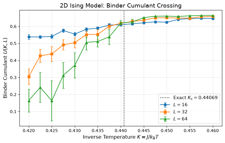
At $T = T_{\mathrm{c}}$ : $U(T_{\mathrm{c}}, L)$ is scale-invariant (all finite-size curves cross at $T_{\mathrm{c}}$ ).

The finite-size scaling relation for $U$ has anomalous dimension $c_2 = 0$ :

U(T, L) = F\left[ (T - T_{\mathrm{c}}) L^{1/\nu} \right] = F\left[ (K - K_{\mathrm{c}}) L^{c_1} \right]

(4)

with exact 2D exponent $\nu = 1 \implies c_1 = 1.0$ .

import numpy as np
import matplotlib.pyplot as plt
import time
import jaxfss

2. Vectorized Checkerboard Metropolis Monte Carlo¶

In a square lattice, sites can be partitioned into two independent sublattices (like black and white squares of a chessboard: $(x + y) \pmod 2 == 0$ and $(x + y) \pmod 2 == 1$ ).

Because nearest neighbors of any “even” site are strictly “odd” sites, all even sites can be updated simultaneously in parallel without race conditions, followed by updating all odd sites.

def simulate_ising_chain(
    L: int,
    inv_T: float,
    n_thermalization: int = 500,
    n_measurements: int = 2000,
    sample_interval: int = 5,
    seed: int = 0,
) -> np.ndarray:
    """Sample magnetization M = sum(sigma) using vectorized checkerboard Metropolis."""
    rng = np.random.default_rng(seed)
    spins = rng.choice([-1, 1], size=(L, L)).astype(np.int8)
    
    # Sublattice masks
    i, j = np.meshgrid(np.arange(L), np.arange(L), indexing="ij")
    mask_even = (i + j) % 2 == 0
    mask_odd = ~mask_even
    
    def sweep():
        for mask in (mask_even, mask_odd):
            # Sum of 4 nearest neighbors with periodic boundary conditions
            nn_sum = (
                np.roll(spins, 1, axis=0)
                + np.roll(spins, -1, axis=0)
                + np.roll(spins, 1, axis=1)
                + np.roll(spins, -1, axis=1)
            )
            dE = 2 * spins * nn_sum
            # Acceptance probability for dE > 0
            prob = np.exp(-inv_T * dE)
            accept = (dE <= 0) | (rng.random((L, L)) < prob)
            spins[mask & accept] *= -1

    # Thermalization sweeps
    for _ in range(n_thermalization):
        sweep()

    # Measurement sweeps
    magnetizations = []
    for step in range(n_measurements * sample_interval):
        sweep()
        if step % sample_interval == 0:
            magnetizations.append(float(np.sum(spins)))

    return np.array(magnetizations)

3. Jackknife Error Estimation for Binder Parameter¶

The Binder cumulant $U = 1 - \frac{\langle M^4 \rangle}{3 \langle M^2 \rangle^2}$ is a ratio of non-linear averages. Standard propagation of error is biased, so we use the Jackknife resampling method.

def compute_binder_jackknife(magnetizations: np.ndarray, n_bins: int = 20) -> tuple[float, float]:
    """Compute Binder parameter and statistical error using Jackknife resampling with binning."""
    # Group into n_bins blocks to eliminate autocorrelation
    n_total = len(magnetizations)
    bin_size = n_total // n_bins
    m_binned = magnetizations[: n_bins * bin_size].reshape(n_bins, bin_size)
    
    # Bin averages of M^2 and M^4
    m2_bins = np.mean(m_binned**2, axis=1)
    m4_bins = np.mean(m_binned**4, axis=1)
    
    # Overall averages
    m2_mean = np.mean(m2_bins)
    m4_mean = np.mean(m4_bins)
    u_full = 1.0 - m4_mean / (3.0 * (m2_mean**2))
    
    # Jackknife pseudo-values (leaving out one bin at a time)
    u_jack = []
    for b in range(n_bins):
        m2_sub = (np.sum(m2_bins) - m2_bins[b]) / (n_bins - 1)
        m4_sub = (np.sum(m4_bins) - m4_bins[b]) / (n_bins - 1)
        u_jack.append(1.0 - m4_sub / (3.0 * (m2_sub**2)))
        
    u_jack = np.array(u_jack)
    # Jackknife standard error formula
    u_err = np.sqrt((n_bins - 1) * np.mean((u_jack - np.mean(u_jack)) ** 2))
    return float(u_full), float(u_err)

4. Multi-Size Simulation and Binder Crossing¶

We simulate three lattice sizes $L \in \{16, 32, 64\}$ over a grid of inverse temperatures $K = J / k_{\mathrm{B}} T$ around $K_{\mathrm{c}} \approx 0.4406868$ .

L_list = [16, 32, 64]
inv_T_values = np.linspace(0.42, 0.46, 17)

results = {}
print("Running 2D Ising simulation...")
t_start = time.time()

for L in L_list:
    u_vals, u_errs = [], []
    for k_idx, inv_T in enumerate(inv_T_values):
        m_chain = simulate_ising_chain(
            L=L,
            inv_T=inv_T,
            n_thermalization=400,
            n_measurements=1500,
            sample_interval=3,
            seed=100 * L + k_idx,
        )
        u, u_err = compute_binder_jackknife(m_chain, n_bins=15)
        u_vals.append(u)
        u_errs.append(u_err)
    results[L] = (np.array(u_vals), np.array(u_errs))
    print(f"  L = {L:2d} completed in {time.time() - t_start:.2f}s")

print(f"Total simulation completed in {time.time() - t_start:.2f}s.")

Running 2D Ising simulation...

  L = 16 completed in 4.07s

  L = 32 completed in 9.95s

  L = 64 completed in 21.97s
Total simulation completed in 21.97s.

Plot the Binder ratio curves. All curves cross at the critical coupling $K_{\mathrm{c}} \approx 0.4406868$ .

plt.figure(figsize=(7.5, 4.8))
markers = ["o", "s", "^"]
K_c_exact = 0.5 * np.log(1 + np.sqrt(2))

for (L, (u_vals, u_errs)), m in zip(results.items(), markers):
    plt.errorbar(inv_T_values, u_vals, yerr=u_errs, fmt=f"{m}-", label=f"$L = {L}$", capsize=3, lw=1.5)

plt.axvline(K_c_exact, color="black", linestyle=":", label=f"Exact $K_{{\mathrm{{c}}}} = {K_c_exact:.5f}$")
plt.xlabel(r"Inverse Temperature $K = J / k_{\mathrm{B}} T$", fontsize=12)
plt.ylabel(r"Binder Cumulant $U(K, L)$", fontsize=12)
plt.title("2D Ising Model: Binder Cumulant Crossing", fontsize=14)
plt.legend(fontsize=11)
plt.grid(True, alpha=0.3)
plt.tight_layout()
plt.show()

<>:8: SyntaxWarning: invalid escape sequence '\m'
<>:8: SyntaxWarning: invalid escape sequence '\m'
/var/folders/g6/3yjn6zvx14s3q4k28w8d78fw0000gn/T/ipykernel_2412/1662117723.py:8: SyntaxWarning: invalid escape sequence '\m'
  plt.axvline(K_c_exact, color="black", linestyle=":", label=f"Exact $K_{{\mathrm{{c}}}} = {K_c_exact:.5f}$")

5. Exporting Dataset for `jaxfss`¶

We save our simulated Binder cumulant data to ising_custom.txt in the standard tabular format:

L  K  U  U_err

output_rows = []
for L, (u_vals, u_errs) in results.items():
    for k_val, u, err in zip(inv_T_values, u_vals, u_errs):
        output_rows.append([L, k_val, u, err])

output_data = np.array(output_rows)
output_path = "ising_custom.txt"

np.savetxt(
    output_path,
    output_data,
    fmt=["%d", "%.8f", "%.8f", "%.8f"],
    header="L K U U_err"
)
print(f"Saved {len(output_data)} rows to {output_path}.")

# Verify loading with jaxfss
loaded_dataset = jaxfss.CriticalData.from_file(output_path)
print(f"Successfully loaded into jaxfss: {loaded_dataset}")
print(f"System sizes in dataset: {np.unique(loaded_dataset.Ls)}")

Saved 51 rows to ising_custom.txt.

Successfully loaded into jaxfss: jaxfss.CriticalData(n_data=51)
System sizes in dataset: [16. 32. 64.]

Summary¶

We have implemented a fast, vectorized 2D Ising Metropolis Monte Carlo simulation, computed Binder cumulants with Jackknife error estimates, verified the universal curve crossing at $T_{\mathrm{c}}$ , and exported the data ready for jaxfss Finite-Size Scaling analysis.